Visulization and Analysis

1. Overview of Ethiopia under COVID-19

- Death New Count and Positive Cases Count

The Trends of Death New Count and Positive Cases Count for Reported Date

This plot shows the trends of people's death new count and positive COVID-19 cases count from December 31, 2019, to September 08, 2020. The orange area represents the death new count, and the brown line represents the positive new cases count. The plot numbers are the death count, and positive cases count on September 08, 2020. These two trends have a similar tendency, which shows that COVID-19 is one of the death count's main factors.

- Positive New Cases Count

Difference in Positive New Cases Count Based on the Previous Day

This plot shows the trend of difference in people's positive new cases counts for Ethiopia's report date day. We can see the case started during mid-March, and the changing rate stayed constant for around two months. The differences in positive new cases count based on the previous day became obvious near July 2020. There are several significant differences around every other two weeks.

Moreover, the most significant difference appeared in early August. Since we do not know the exact date of government measures during COVID-19, we think there are several possibilities. One might be that Covid-19 reached the outbreak period, or the government measures encouraged and supported medical institutions for the nucleic acid test.

Up to September 2020, the increasing rate of positive new cases in Ethiopia still had apparent differences based on the previous days. However, it seemed to be controlled and more negative numbers, which means fewer positive new cases counted on those dates, represented compared to before.

- Death New Count and Positive Cases Count

The Plot of Death New Count for Reported Data in Ethiopia

This plot shows the number of new death count for the reported date from January 2020 to September 2020. As we can see, there was very few death during the first half of 2020. It had a small fluctuation between June and July, but we do not know if the change was due to the Covid 19 or other reasons. When it goes to August, there was a peak; Covid 19 may be one factor since there was a peak on the new positive cases count around the same time. Then the food industry would be affected because of the loss in the labor force.

Furthermore, it would increase the cost of food production, food transportation, and food storage. As a result, people who live in Ethiopia could not have enough high-quality food supply, which will lead to more death in the country. Hence, we can see that Covid 19 is one factor that aggravates food security problems.

2. Government's Measures

- Overview of measures

We made a histogram with the variables of government measures. Based on the plot, the top three measures are limit public gathering, economic measures and isolation, and quarantine policies.

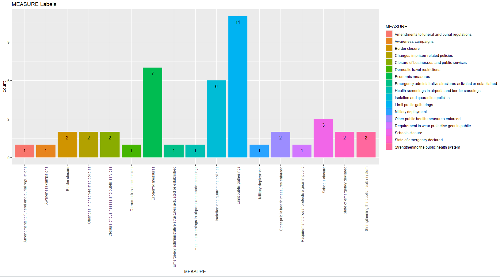
Histogram

- Category

The measures above have specific classifications, which we show in a classification histogram.

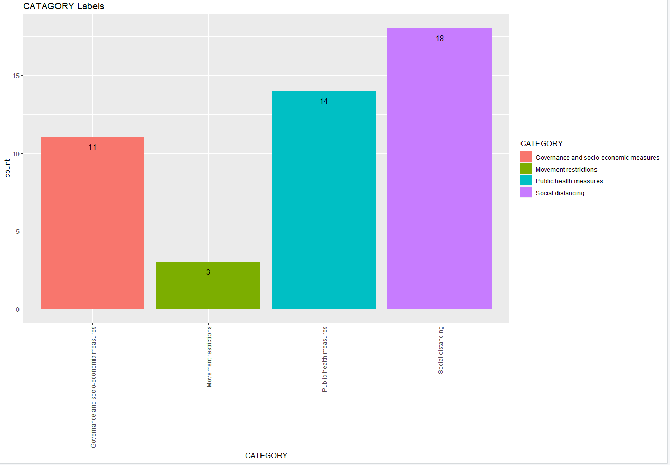
Classification Histogram

According to the histogram, the most commonly used measure classifications are social distancing, limit public gathering and isolation, and quarantine policies. The government uses people's isolation as the primary method to control the epidemic, supplemented by other measures.

Clik to view R code

- Wordcloud

We can also find out what the government's specific actions are to deal with COVID-19 by creating the word cloud for explanatory comments.

Worldcloud

Based on the word cloud, we can see that the government plays an essential role during COVID-19. Facilities, quarantine, transport, masks are all key factors in government measures.

Clik to view Python code

3. Economy and Food

- Correlation

To determine which variables are positively correlated with others. We plot a heatmap with correlation coefficients (>=0 and <= 1). Observed that the deeper color each block has, the higher correlation it has with other variables.

Click right corner to enlarge the plot

Link to the plot

By inspecting the heatmap, we can see the correlation coefficients between each pair of variables are pretty high, so we cannot easily decide which variables to remove and keep. To better the model, we need to figure it out by linear regression.

- Feature Selection

Then we can select the features without highly correlated variables with backward selection in linear regression. We selected six variables as predictors based on adjusted R-square.

Including:

● Proportion of population under global poverty line

● Volatility of agricultural production

● Protein quality

● Ability to store food safely

● Natural Disaster (or disease) Disbursement

● Agriculture expenditure in GDP

linear model

Clik to view Python code

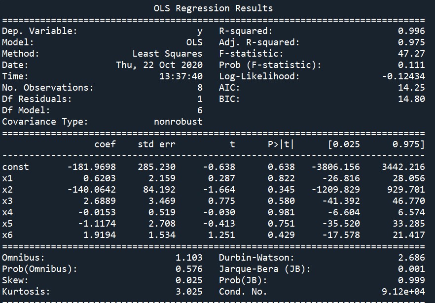
Observed for some selected variables, the p-value in the linear model is high (>0.05). The reason to keep such variables in the model is that this model has only 8 rows and is limited to further optimization.

Thus, we get the linear model:

Prevalence of undernourishment population = -181.9698

+ 0.6203*Proportion of population under global poverty line (X1)

-140.0642*Volatility of agricultural production(X2)

+2.6889*Protein quality(X3)

-0.0153*Ability to store food safely(X4)

-1.1174*Natural Disaster (or disease) Disbursement(X5)

+1.9194*Agriculture expenditure in GDP(X6)

Among those variables, Covid-19 is included in ‘Natural Disaster (or disease) Disbursement’. We can predict the proportion of undernourishment population in 2020 by the total disbursement of Covid-19 and other data. The figure below is the scatter plot and histogram of predictors each year.

Click right corner to enlarge the plot

Link to the plot

Click right corner to enlarge the plot

Link to the plot

By clicking each year, we can explore the values of predictors in that year. And by clicking each predictor, we can observe the change of it from 2012 to 2019. For example, since “Prevalence of undernourishment population” is decreasing from 2012 to 2019, so does “Agriculture expenditure in GDP”; we can conclude that they have a positive correlation.

Thus, if the government expenditure on agriculture increases during the COVID-19, it indicates more people will suffer undernourishment.

4. Exposure Risk Score

Ethiopia has 11 regions and more than 600 small districts. First, we make a map to display the average total exposure score of each region.

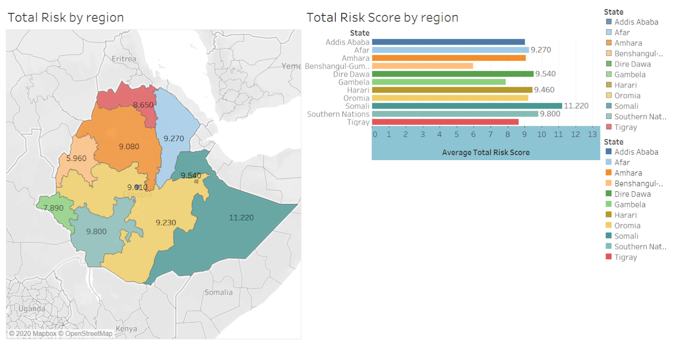
As we can see, the region has the highest risk score is in the east, the areas have medium to high risk score is clustered in the middle, the regions that have low-risk score are in the west. Most regions have a risk score of around 9 to 10. Then we want to explore the connection between socio-economic vulnerability and average total risk.

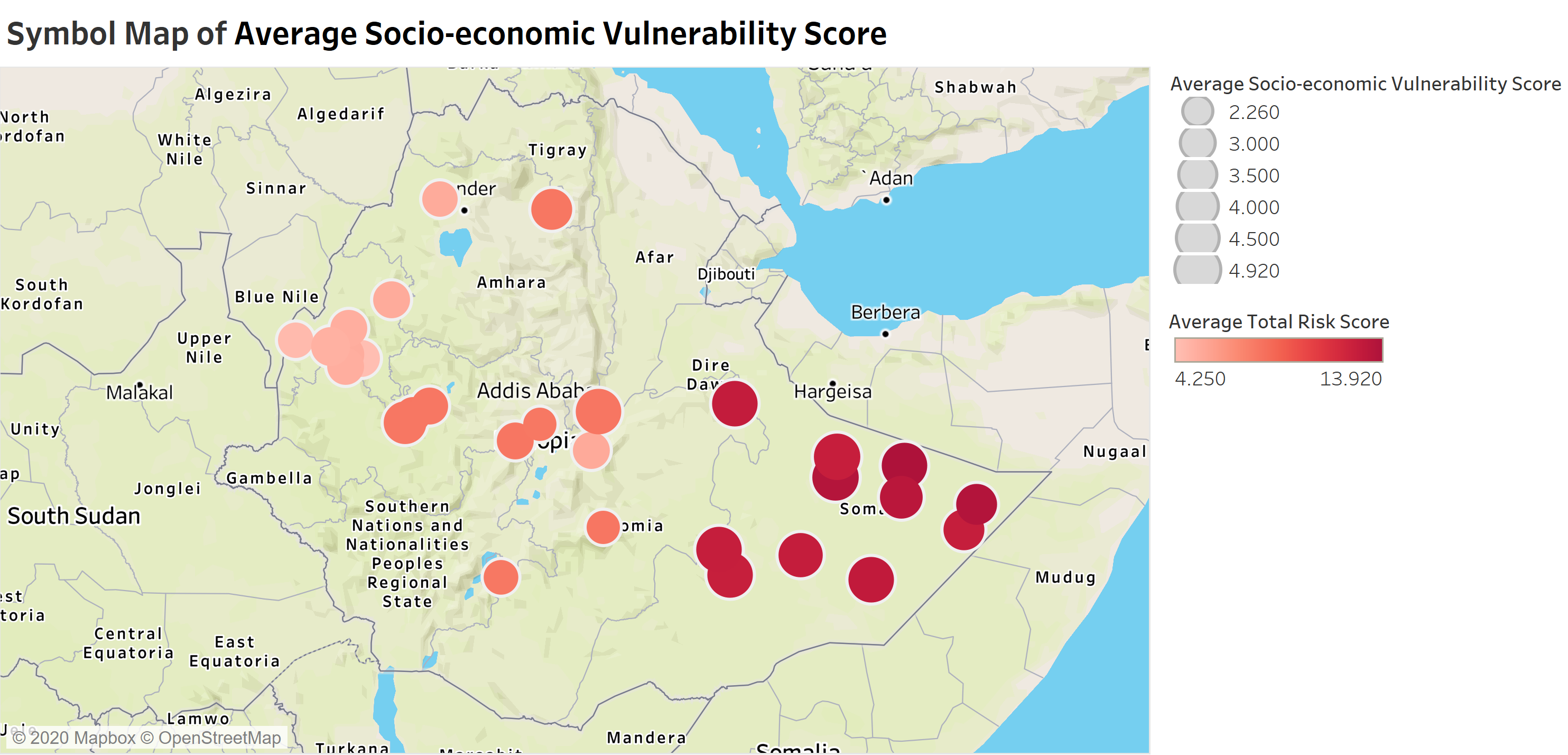
Symbol Map of Average Socio-Economic Vulnerability Score by Districts

Since there are more than 600 small districts, we make 30 samples. 10 has a low total risk score, 10 has a medium total risk score, and others have a high total risk score. The bubble size represents the average socio-economic vulnerability score, and the color represents the total risk score.

This graph clearly shows that districts with high socio-economic vulnerability scores also have a high total average risk score, which indicates that people who live there can be affected by COVID-19 more easily than districts in other areas.

Moreover, an interesting finding is that more population does not indicate people in that area are much easier to be affected by COVID-19.

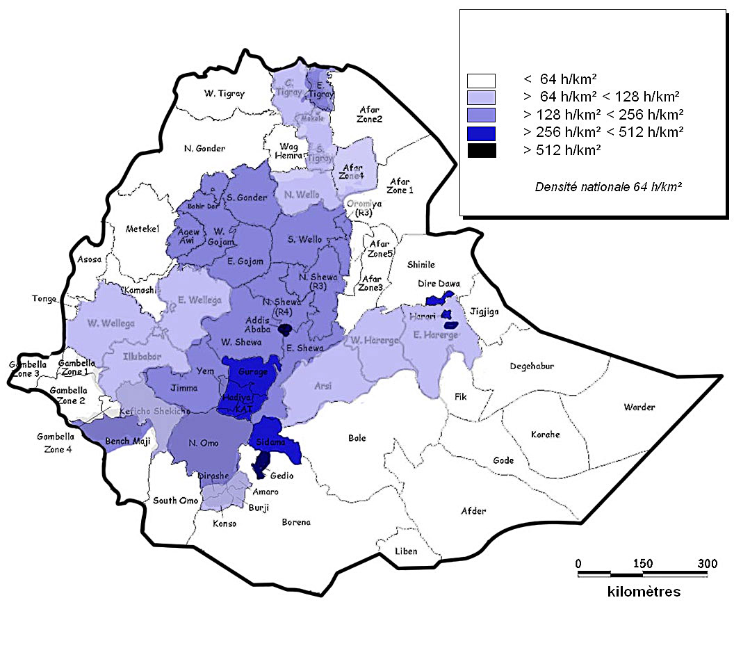
Ethiopia population density map

It seems counter intuitive, but it is what our data shows. Above is the Ethiopia population density map. Based on the graph, most of the population is clustered in the middle and west areas. There are not so many people in the east area. However, the previous analysis shows that the east region has the highest total risk score. Thus, a high population does not imply a high risk of being infected by COVID-19.